In [15]:

!git clone https://github.com/acmbpdc/ml-bootcamp-2023.git

!git clone https://github.com/acmbpdc/ml-bootcamp-2023.git

fatal: destination path 'ml-bootcamp-2023' already exists and is not an empty directory.

In [16]:

!cp /content/ml-bootcamp-2023/docs/04-evaluating-and-tuning/heart_v2.csv /content

!cp /content/ml-bootcamp-2023/docs/04-evaluating-and-tuning/heart_v2.csv /content

Evaluating and Tuning Models¶

Summary:¶

• Evaluating the performance of models
• Metrics to measure the performance of models
• Hyperparameter tuning of the model, to achieve maximum accuracy

Metrics to Evaluate Machine Learning models¶

The Train/Test/Validation split¶

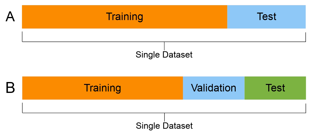
The most important thing you can do to properly evaluate your model is to not train the model on the entire dataset. A typical train/test/validation split would be to use 60% of the data for training set, 20% of the data for test set, and 20% of the data for validation set.

• Train Set: This subset of the dataset is used for training the parameters of your machine learning model, and repetitively iterating and improving the model weights. The accuracy of the model on this subset of dataset is called Train Accuracy.

• Test Set: This subset of the dataset is used for checking the accuracy of the model on new, unseen data while the training process is ongoing. The accuracy of the model on this subset is called Test Accuracy, and is used for tuning the hyperparameters (learning rate, batch size, number of epochs, optimizer, etc), to improve the accuracy.

• Validation Accuracy: (optional) Now, since we have tuned the hyperparameters to the Test Set to give good accuracy, but maybe the hyperparameters chosen don't work for another new set of data. So, as a final check we can also use another subset of the dataset called Validation Set, to check if the model is generalising well.

Note: In case you have a small dataset and do not want to make a separate validation set (as that would mean lesser data for training), you can use train accuracy and test accuracy, if the train and test accuracy are within 4-5% of each other, it means that the model is working well for new data.

Classification Metrics¶

When performing classification predictions, there's four types of outcomes that could occur.

• True Positives: When you predict an observation belongs to a class and it actually does belong to that class.
• True negatives: when you predict an observation does not belong to a class and it actually does not belong to that class.
• False positives: When you predict an observation belongs to a class when in reality it does not.
• False negatives: When you predict an observation does not belong to a class when in fact it does.

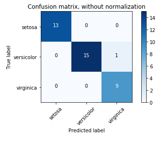
These four outcomes are often plotted on a Confusion Matrix.

Confusion Matrix: It is a performance measurement for machine learning classification problem where output can be two or more classes. It is a table with 4 different combinations of predicted and actual values.

The following confusion matrix is an example for the case of binary classification. You would generate this matrix after making predictions on your test data and then identifying each prediction as one of the four possible outcomes described above.

You can also extend this confusion matrix to plot multi-class classification predictions. The following is an example confusion matrix for classifying observations from the Iris flower dataset.

The three main metrics used to evaluate a classification model are:

• Accuracy: The percentage of correct predictions for the test data. It can be calculated easily by dividing the number of correct predictions by the number of total predictions.
  Accuracy = (TP+TN)/Total
• Precision: The fraction of correct predictions (true positives) among all of the data points which were predicted to belong in a certain class.
  Precision = (TP)/(TP+FP)
• Recall: The fraction of data points which were predicted to belong to a class with respect to all of the data points that truly belong in the class.
  Recall = (TP)/(TP+FN)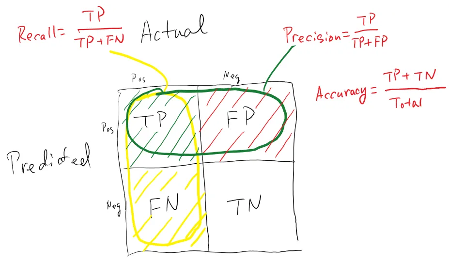
  
  

Why do we use Precision and Recall?¶

• Precision and recall are useful in cases where classes aren't evenly distributed.
• The common example is for developing a classification algorithm that predicts whether or not someone has a disease. If only a small percentage of the population (let's say 1%) has this disease, we could build a classifier that always predicts that the person does not have the disease, we would have built a model which is 99% accurate and 0% useful.
• If we had checked the recall of the model described above, this could have been easily diagnosed.
• Recall ensures that we're not overlooking the people who have the disease, while precision ensures that we're not misclassifying too many people as having the disease when they don't.

A metric called F1 Score is used to represent Precision and recall together.

F1 Score = Precision*Recall/ (Precision+Recall)

Regression Metrics¶

Evaluation metrics for regression models are quite different than the above metrics we discussed for classification models because we are now predicting in a continuous range instead of a discrete number of classes

• Mean Squared Error: or MSE for short, is a popular error metric for regression problems. It is also an important loss function for algorithms fit or optimized using the least squares framing of a regression problem. Here “least squares” refers to minimizing the mean squared error between predictions and expected values. The MSE is calculated as the mean or average of the squared differences between predicted and expected target values in a dataset.

  

• Root Mean Squared Error: or RMSE, is an extension of the mean squared error. Importantly, the square root of the error is calculated, which means that the units of the RMSE are the same as the original units of the target value that is being predicted. Thus, it may be common to use MSE loss to train a regression predictive model, and to use RMSE to evaluate and report its performance.

• Mean Absolute Error:or MAE, is a popular metric because, like RMSE, the units of the error score match the units of the target value that is being predicted. Unlike the RMSE, the changes in MAE are linear and therefore intuitive.That is, MSE and RMSE punish larger errors more than smaller errors, inflating or magnifying the mean error score. This is due to the square of the error value. The MAE does not give more or less weight to different types of errors and instead the scores increase linearly with increases in error

Overfitting vs Underfitting (Bias vs Variance)¶

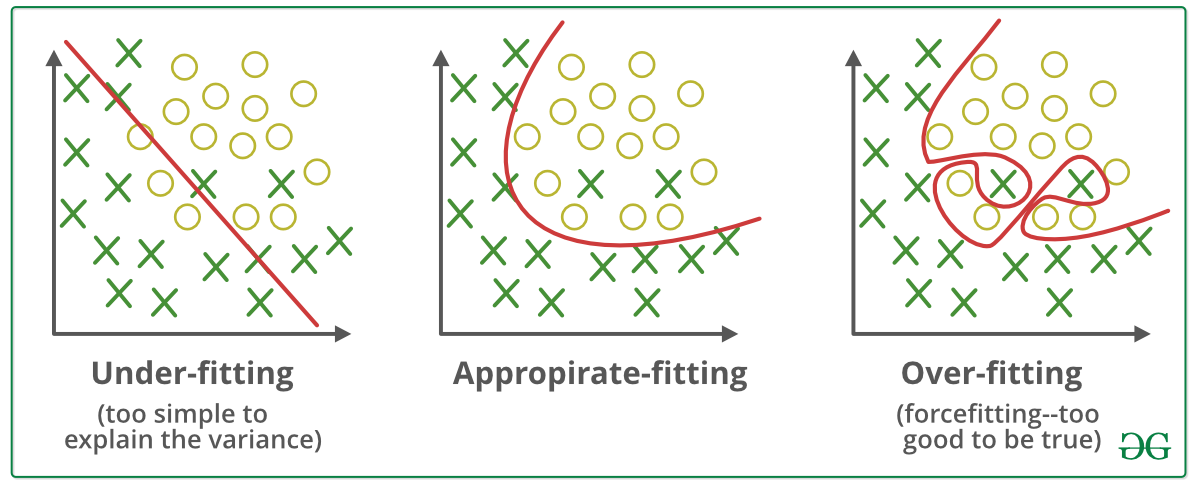
• Overfitting (Bias) refers to a model that models the training data too well. Overfitting happens when a model learns the detail and noise in the training data to the extent that it negatively impacts the performance of the model on new data. This means that the noise or random fluctuations in the training data is picked up and learned as concepts by the model. The problem is that these concepts do not apply to new data and negatively impact the models ability to generalize.
  Signs of Overfitting: Your train accuracy is high, but your test accuracy is much lower
• Underfitting refers to a model that can neither model the training data nor generalize to new data. An underfit machine learning model is not a suitable model and will be obvious as it will have poor performance on the training data. Underfitting is often not discussed as it is easy to detect given a good performance metric. The remedy is to move on and try alternate machine learning algorithms
  Signs of Underfitting: Both your train and test accuracy are low

Why does overfitting occur?:¶

Overfitting happens due to several reasons, such as:

• The training data size is too small and does not contain enough data samples to accurately represent all possible input data values.
• The training data contains large amounts of irrelevant information, called noisy data.
• The model trains for too long on a single sample set of data.

Strategies to overcome overfitting¶

You can prevent overfitting by diversifying and scaling your training data set or using some other data science strategies, like those given below.

• Early stopping Early stopping pauses the training phase before the machine learning model learns the noise in the data. However, getting the timing right is important; else the model will still not give accurate results.

• Pruning You might identify several features or parameters that impact the final prediction when you build a model. Feature selection—or pruning—identifies the most important features within the training set and eliminates irrelevant ones

• Regularization Regularization is a collection of training/optimization techniques that seek to reduce overfitting. These methods try to eliminate those factors that do not impact the prediction outcomes by grading features based on importance

• Ensembling Ensembling combines predictions from several separate machine learning algorithms. Some models are called weak learners because their results are often inaccurate. Ensemble methods combine all the weak learners to get more accurate results

• Data augmentation Data augmentation is a machine learning technique that changes the sample data slightly every time the model processes it. You can do this by changing the input data in small ways. When done in moderation, data augmentation makes the training sets appear unique to the model and prevents the model from learning their characteristics

Hyperparameter Tuning¶

What are Hyperparameters?¶

• Hyperparameters are the parameters that cannot be estimated by the model itself and you need you specify them manually. These parameters affect your model in many ways for a specific set of data.
• For your model to perform best you have choose the best set of hyperparameters.
• For example, Max Depth in Decision Tree and Learning rate in Deep Neural Network. These hyperparameters have a direct effect on whether your model will be Underfitting or Overfitting. The Bias Variance trade-off is heavily reliant on hyperparameter tuning.

What is Hyperparameter Tuning?¶

In most of the ML models there will be multiple hyperparameters. Choosing the best combination requires an understanding of the model's parameters and the business problem you’re trying to tackle. So before doing anything you have to know the hyperparameters of the models and their importance.

To get the best hyperparameter the two step procedure is followed .

• For each combination of hyperparameters the model is evaluated
• The combination that gives the best performing model are selected as optimal hyperparameters.

So, put simply, choosing the best set of hyperparameters that result in the best model is called Hyperparameter Tuning.

Methods for Tuning Hyperparameters¶

Now that we understand what hyperparameters are and the importance of tuning them, we need to know how to choose their optimal values. We can find these optimal hyperparameter values using manual or automated methods.

When tuning hyperparameters manually, we typically start using the default recommended values or rules of thumb, then search through a range of values using trial-and-error. But manual tuning is a tedious and time-consuming approach. It isn’t practical when there are many hyperparameters with a wide range.

Automated hyperparameter tuning methods use an algorithm to search for the optimal values. Some of today’s most popular automated methods are grid search, random search, and Bayesian optimization. Let’s explore these methods in detail.

• Grid Search:
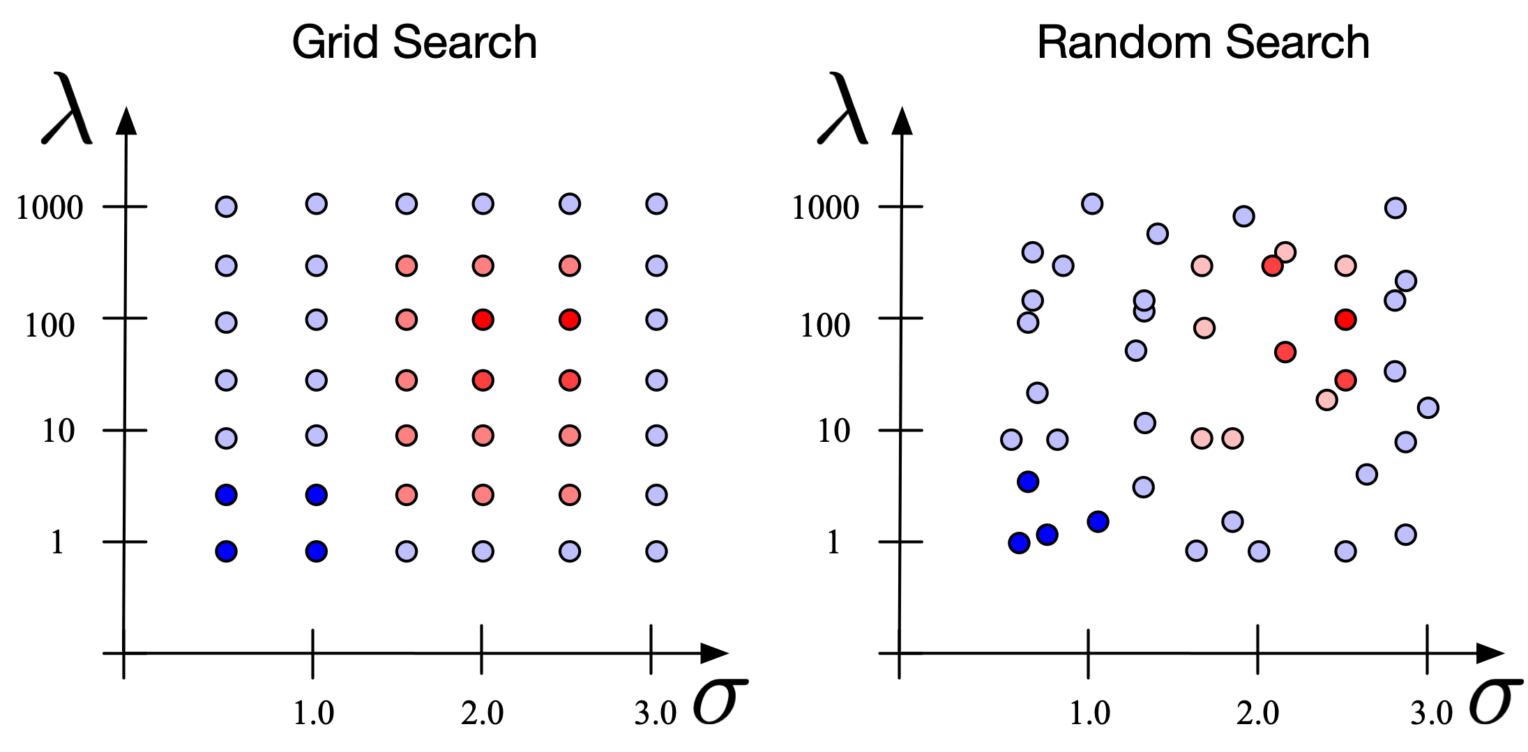
  • Grid search is a sort of “brute force” hyperparameter tuning method. We create a grid of possible discrete hyperparameter values then fit the model with every possible combination. We record the model performance for each set then select the combination that has produced the best performance.
  • Grid search is an exhaustive algorithm that can find the best combination of hyperparameters. However, the drawback is that it’s slow. Fitting the model with every possible combination usually requires a high computation capacity and significant time
    

• Random search:
  • The random search method (as its name implies) chooses values randomly rather than using a predefined set of values like the grid search method.
  • Random search tries a random combination of hyperparameters in each iteration and records the model performance. After several iterations, it returns the mix that produced the best result.
  • Random search is appropriate when we have several hyperparameters with relatively large search domains.
  • The benefit is that random search typically requires less time than grid search to return a comparable result, but the drawback is that the result may not be the best possible hyperparameter combination.

Hyperparameter tuning example for Decision Trees¶

In [17]:

# Importing the required libraries
import pandas as pd, numpy as np
import matplotlib.pyplot as plt, seaborn as sns
%matplotlib inline

# Importing the required libraries import pandas as pd, numpy as np import matplotlib.pyplot as plt, seaborn as sns %matplotlib inline

In [18]:

# Reading the csv file and putting it into 'df' object.
df = pd.read_csv("/content/heart_v2.csv")

# Reading the csv file and putting it into 'df' object. df = pd.read_csv("/content/heart_v2.csv")

In [19]:

df.columns

df.columns

Out[19]:

Index(['age', 'sex', 'BP', 'cholestrol', 'heart disease'], dtype='object')

In [20]:

df.head()

df.head()

Out[20]:

	age	sex	BP	cholestrol	heart disease
0	70	1	130	322	1
1	67	0	115	564	0
2	57	1	124	261	1
3	64	1	128	263	0
4	74	0	120	269	0

In [21]:

df.shape

df.shape

Out[21]:

(270, 5)

In [22]:

df.info()

df.info()

<class 'pandas.core.frame.DataFrame'>
RangeIndex: 270 entries, 0 to 269
Data columns (total 5 columns):
 #   Column         Non-Null Count  Dtype
---  ------         --------------  -----
 0   age            270 non-null    int64
 1   sex            270 non-null    int64
 2   BP             270 non-null    int64
 3   cholestrol     270 non-null    int64
 4   heart disease  270 non-null    int64
dtypes: int64(5)
memory usage: 10.7 KB

EDA¶

In [23]:

plt.figure(figsize = (10,5))
ax= sns.violinplot(df['age'])
plt.show()

plt.figure(figsize = (10,5)) ax= sns.violinplot(df['age']) plt.show()

In [24]:

plt.figure(figsize = (15,5))
ax= sns.countplot(df['sex'])
for p in ax.patches:
    ax.annotate(str(p.get_height()), (p.get_x() * 1.01 , p.get_height() * 1.01))
plt.xticks(rotation = 45)
plt.show()

plt.figure(figsize = (15,5)) ax= sns.countplot(df['sex']) for p in ax.patches: ax.annotate(str(p.get_height()), (p.get_x() * 1.01 , p.get_height() * 1.01)) plt.xticks(rotation = 45) plt.show()

In [25]:

plt.figure(figsize = (10,5))
ax= sns.violinplot(df['BP'])
plt.show()

plt.figure(figsize = (10,5)) ax= sns.violinplot(df['BP']) plt.show()

In [26]:

percentiles = df['BP'].quantile([0.05,0.95]).values
df['BP'][df['BP'] <= percentiles[0]] = percentiles[0]
df['BP'][df['BP'] >= percentiles[1]] = percentiles[1]

percentiles = df['BP'].quantile([0.05,0.95]).values df['BP'][df['BP'] <= percentiles[0]] = percentiles[0] df['BP'][df['BP'] >= percentiles[1]] = percentiles[1]

In [27]:

plt.figure(figsize = (10,5))
ax= sns.violinplot(df['BP'])
plt.show()

plt.figure(figsize = (10,5)) ax= sns.violinplot(df['BP']) plt.show()

In [28]:

plt.figure(figsize = (10,5))
ax= sns.violinplot(df['cholestrol'])
plt.show()

plt.figure(figsize = (10,5)) ax= sns.violinplot(df['cholestrol']) plt.show()

In [29]:

percentiles = df['cholestrol'].quantile([0.05,0.95]).values
df['cholestrol'][df['cholestrol'] <= percentiles[0]] = percentiles[0]
df['cholestrol'][df['cholestrol'] >= percentiles[1]] = percentiles[1]

percentiles = df['cholestrol'].quantile([0.05,0.95]).values df['cholestrol'][df['cholestrol'] <= percentiles[0]] = percentiles[0] df['cholestrol'][df['cholestrol'] >= percentiles[1]] = percentiles[1]

<ipython-input-29-7853381cafe8>:2: SettingWithCopyWarning: 
A value is trying to be set on a copy of a slice from a DataFrame

See the caveats in the documentation: https://pandas.pydata.org/pandas-docs/stable/user_guide/indexing.html#returning-a-view-versus-a-copy
  df['cholestrol'][df['cholestrol'] <= percentiles[0]] = percentiles[0]
<ipython-input-29-7853381cafe8>:3: SettingWithCopyWarning: 
A value is trying to be set on a copy of a slice from a DataFrame

See the caveats in the documentation: https://pandas.pydata.org/pandas-docs/stable/user_guide/indexing.html#returning-a-view-versus-a-copy
  df['cholestrol'][df['cholestrol'] >= percentiles[1]] = percentiles[1]

In [30]:

plt.figure(figsize = (10,5))
ax= sns.violinplot(df['cholestrol'])
plt.show()

plt.figure(figsize = (10,5)) ax= sns.violinplot(df['cholestrol']) plt.show()

In [31]:

plt.figure(figsize = (15,5))
ax= sns.countplot(df['heart disease'])
for p in ax.patches:
    ax.annotate(str(p.get_height()), (p.get_x() * 1.01 , p.get_height() * 1.01))
plt.xticks(rotation = 45)
plt.show()

plt.figure(figsize = (15,5)) ax= sns.countplot(df['heart disease']) for p in ax.patches: ax.annotate(str(p.get_height()), (p.get_x() * 1.01 , p.get_height() * 1.01)) plt.xticks(rotation = 45) plt.show()

In [32]:

plt.figure(figsize = (10,5))
sns.violinplot(y = 'age', x = 'heart disease', data = df)
plt.show()

plt.figure(figsize = (10,5)) sns.violinplot(y = 'age', x = 'heart disease', data = df) plt.show()

In [33]:

plt.figure(figsize = (10,5))
ax= sns.countplot(x = "sex", hue = "heart disease", data = df)
for p in ax.patches:
    ax.annotate(str(p.get_height()), (p.get_x() * 1.01 , p.get_height() * 1.01))
plt.xticks(rotation = 90)
plt.show()

plt.figure(figsize = (10,5)) ax= sns.countplot(x = "sex", hue = "heart disease", data = df) for p in ax.patches: ax.annotate(str(p.get_height()), (p.get_x() * 1.01 , p.get_height() * 1.01)) plt.xticks(rotation = 90) plt.show()

In [34]:

plt.figure(figsize = (10,5))
sns.violinplot(y = 'BP', x = 'heart disease', data = df)
plt.show()

plt.figure(figsize = (10,5)) sns.violinplot(y = 'BP', x = 'heart disease', data = df) plt.show()

In [35]:

plt.figure(figsize = (10,5))
sns.violinplot(y = 'cholestrol', x = 'heart disease', data = df)
plt.show()

plt.figure(figsize = (10,5)) sns.violinplot(y = 'cholestrol', x = 'heart disease', data = df) plt.show()

In [36]:

plt.figure(figsize = (10,5))
sns.heatmap(df.corr(), annot = True, cmap="rainbow")
plt.show()

plt.figure(figsize = (10,5)) sns.heatmap(df.corr(), annot = True, cmap="rainbow") plt.show()

In [37]:

df.describe()

df.describe()

Out[37]:

	age	sex	BP	cholestrol	heart disease
count	270.000000	270.000000	270.000000	270.000000	270.000000
mean	54.433333	0.677778	130.824444	247.895185	0.444444
std	9.109067	0.468195	15.387319	42.641693	0.497827
min	29.000000	0.000000	106.900000	177.000000	0.000000
25%	48.000000	0.000000	120.000000	213.000000	0.000000
50%	55.000000	1.000000	130.000000	245.000000	0.000000
75%	61.000000	1.000000	140.000000	280.000000	1.000000
max	77.000000	1.000000	160.000000	326.550000	1.000000

In [38]:

# Putting feature variable to X
X = df.drop('heart disease',axis=1)

# Putting response variable to y
y = df['heart disease']

# Putting feature variable to X X = df.drop('heart disease',axis=1) # Putting response variable to y y = df['heart disease']

In [39]:

from sklearn.model_selection import train_test_split

from sklearn.model_selection import train_test_split

In [40]:

X_train, X_test, y_train, y_test = train_test_split(X, y, train_size=0.6, random_state=50)
X_train.shape, X_test.shape

X_train, X_test, y_train, y_test = train_test_split(X, y, train_size=0.6, random_state=50) X_train.shape, X_test.shape

Out[40]:

((162, 4), (108, 4))

Fitting the decision tree with default hyperparameters, apart from max_depth which is 3 so that we can plot and read the tree.

In [41]:

from sklearn.tree import DecisionTreeClassifier

from sklearn.tree import DecisionTreeClassifier

In [42]:

dt = DecisionTreeClassifier(max_depth=3)
dt.fit(X_train, y_train)

dt = DecisionTreeClassifier(max_depth=3) dt.fit(X_train, y_train)

Out[42]:

DecisionTreeClassifier(max_depth=3)

In a Jupyter environment, please rerun this cell to show the HTML representation or trust the notebook.
On GitHub, the HTML representation is unable to render, please try loading this page with nbviewer.org.

In [43]:

from sklearn import tree
fig = plt.figure(figsize=(25,20))
_ = tree.plot_tree(dt,
                   feature_names=X.columns,
                   class_names=['No Disease', "Disease"],
                   filled=True)

from sklearn import tree fig = plt.figure(figsize=(25,20)) _ = tree.plot_tree(dt, feature_names=X.columns, class_names=['No Disease', "Disease"], filled=True)

Evaluating model performance¶

In [44]:

y_train_pred = dt.predict(X_train)
y_test_pred = dt.predict(X_test)

y_train_pred = dt.predict(X_train) y_test_pred = dt.predict(X_test)

In [45]:

from sklearn.metrics import confusion_matrix, accuracy_score

from sklearn.metrics import confusion_matrix, accuracy_score

In [46]:

print(accuracy_score(y_train, y_train_pred))
confusion_matrix(y_train, y_train_pred)

print(accuracy_score(y_train, y_train_pred)) confusion_matrix(y_train, y_train_pred)

0.7160493827160493

Out[46]:

array([[72, 15],
       [31, 44]])

In [47]:

print(accuracy_score(y_test, y_test_pred))
confusion_matrix(y_test, y_test_pred)

print(accuracy_score(y_test, y_test_pred)) confusion_matrix(y_test, y_test_pred)

0.7037037037037037

Out[47]:

array([[51, 12],
       [20, 25]])

Creating helper functions to evaluate model performance and help plot the decision tree

In [48]:

def get_dt_graph(dt_classifier):
    fig = plt.figure(figsize=(25,20))
    _ = tree.plot_tree(dt_classifier,
                       feature_names=X.columns,
                       class_names=['No Disease', "Disease"],
                       filled=True)

def get_dt_graph(dt_classifier): fig = plt.figure(figsize=(25,20)) _ = tree.plot_tree(dt_classifier, feature_names=X.columns, class_names=['No Disease', "Disease"], filled=True)

In [49]:

def evaluate_model(dt_classifier):
    print("Train Accuracy :", accuracy_score(y_train, dt_classifier.predict(X_train)))
    print("Train Confusion Matrix:")
    print(confusion_matrix(y_train, dt_classifier.predict(X_train)))
    print("-"*50)
    print("Test Accuracy :", accuracy_score(y_test, dt_classifier.predict(X_test)))
    print("Test Confusion Matrix:")
    print(confusion_matrix(y_test, dt_classifier.predict(X_test)))

def evaluate_model(dt_classifier): print("Train Accuracy :", accuracy_score(y_train, dt_classifier.predict(X_train))) print("Train Confusion Matrix:") print(confusion_matrix(y_train, dt_classifier.predict(X_train))) print("-"*50) print("Test Accuracy :", accuracy_score(y_test, dt_classifier.predict(X_test))) print("Test Confusion Matrix:") print(confusion_matrix(y_test, dt_classifier.predict(X_test)))

Without setting any hyper-parameters¶

In [50]:

dt_default = DecisionTreeClassifier(random_state=42)
dt_default.fit(X_train, y_train)

dt_default = DecisionTreeClassifier(random_state=42) dt_default.fit(X_train, y_train)

Out[50]:

DecisionTreeClassifier(random_state=42)

In a Jupyter environment, please rerun this cell to show the HTML representation or trust the notebook.
On GitHub, the HTML representation is unable to render, please try loading this page with nbviewer.org.

In [51]:

gph = get_dt_graph(dt_default)

gph = get_dt_graph(dt_default)

In [52]:

evaluate_model(dt_default)

evaluate_model(dt_default)

Train Accuracy : 1.0
Train Confusion Matrix:
[[87  0]
 [ 0 75]]
--------------------------------------------------
Test Accuracy : 0.7222222222222222
Test Confusion Matrix:
[[46 17]
 [13 32]]

Controlling the depth of the tree¶

In [53]:

dt_depth = DecisionTreeClassifier(max_depth=3)
dt_depth.fit(X_train, y_train)

dt_depth = DecisionTreeClassifier(max_depth=3) dt_depth.fit(X_train, y_train)

Out[53]:

DecisionTreeClassifier(max_depth=3)

In a Jupyter environment, please rerun this cell to show the HTML representation or trust the notebook.
On GitHub, the HTML representation is unable to render, please try loading this page with nbviewer.org.

In [54]:

gph = get_dt_graph(dt_depth)

gph = get_dt_graph(dt_depth)

In [55]:

evaluate_model(dt_depth)

evaluate_model(dt_depth)

Train Accuracy : 0.7160493827160493
Train Confusion Matrix:
[[72 15]
 [31 44]]
--------------------------------------------------
Test Accuracy : 0.7037037037037037
Test Confusion Matrix:
[[51 12]
 [20 25]]

Specifying minimum samples before split¶

In [56]:

dt_min_split = DecisionTreeClassifier(min_samples_split=20)
dt_min_split.fit(X_train, y_train)

dt_min_split = DecisionTreeClassifier(min_samples_split=20) dt_min_split.fit(X_train, y_train)

Out[56]:

DecisionTreeClassifier(min_samples_split=20)

In a Jupyter environment, please rerun this cell to show the HTML representation or trust the notebook.
On GitHub, the HTML representation is unable to render, please try loading this page with nbviewer.org.

In [57]:

gph = get_dt_graph(dt_min_split)

gph = get_dt_graph(dt_min_split)

In [58]:

evaluate_model(dt_min_split)

evaluate_model(dt_min_split)

Train Accuracy : 0.7839506172839507
Train Confusion Matrix:
[[68 19]
 [16 59]]
--------------------------------------------------
Test Accuracy : 0.7222222222222222
Test Confusion Matrix:
[[47 16]
 [14 31]]

Specifying minimum samples in leaf node¶

In [59]:

dt_min_leaf = DecisionTreeClassifier(min_samples_leaf=20, random_state=42)
dt_min_leaf.fit(X_train, y_train)

dt_min_leaf = DecisionTreeClassifier(min_samples_leaf=20, random_state=42) dt_min_leaf.fit(X_train, y_train)

Out[59]:

DecisionTreeClassifier(min_samples_leaf=20, random_state=42)

In a Jupyter environment, please rerun this cell to show the HTML representation or trust the notebook.
On GitHub, the HTML representation is unable to render, please try loading this page with nbviewer.org.

In [60]:

gph = get_dt_graph(dt_min_leaf)

gph = get_dt_graph(dt_min_leaf)

In [61]:

evaluate_model(dt_min_leaf)

evaluate_model(dt_min_leaf)

Train Accuracy : 0.6728395061728395
Train Confusion Matrix:
[[70 17]
 [36 39]]
--------------------------------------------------
Test Accuracy : 0.7037037037037037
Test Confusion Matrix:
[[53 10]
 [22 23]]

Using Entropy instead of Gini¶

In [62]:

dt_min_leaf_entropy = DecisionTreeClassifier(min_samples_leaf=20, random_state=42, criterion="entropy")
dt_min_leaf_entropy.fit(X_train, y_train)

dt_min_leaf_entropy = DecisionTreeClassifier(min_samples_leaf=20, random_state=42, criterion="entropy") dt_min_leaf_entropy.fit(X_train, y_train)

Out[62]:

DecisionTreeClassifier(criterion='entropy', min_samples_leaf=20,
                       random_state=42)

In a Jupyter environment, please rerun this cell to show the HTML representation or trust the notebook.
On GitHub, the HTML representation is unable to render, please try loading this page with nbviewer.org.

In [63]:

gph = get_dt_graph(dt_min_leaf_entropy)

gph = get_dt_graph(dt_min_leaf_entropy)

In [64]:

evaluate_model(dt_min_leaf_entropy)

evaluate_model(dt_min_leaf_entropy)

Train Accuracy : 0.6728395061728395
Train Confusion Matrix:
[[70 17]
 [36 39]]
--------------------------------------------------
Test Accuracy : 0.7037037037037037
Test Confusion Matrix:
[[53 10]
 [22 23]]

Hyper-parameter tuning¶

In [65]:

dt = DecisionTreeClassifier(random_state=42)

dt = DecisionTreeClassifier(random_state=42)

In [66]:

from sklearn.model_selection import GridSearchCV

from sklearn.model_selection import GridSearchCV

In [67]:

# Create the parameter grid based on the results of random search 
params = {
    'max_depth': [2, 3, 5, 10, 20],
    'min_samples_leaf': [5, 10, 20, 50, 100],
    'criterion': ["gini", "entropy"]
}

# Create the parameter grid based on the results of random search params = { 'max_depth': [2, 3, 5, 10, 20], 'min_samples_leaf': [5, 10, 20, 50, 100], 'criterion': ["gini", "entropy"] }

In [68]:

# grid_search = GridSearchCV(estimator=dt, 
#                            param_grid=params, 
#                            cv=4, n_jobs=-1, verbose=1, scoring = "f1")

# grid_search = GridSearchCV(estimator=dt, # param_grid=params, # cv=4, n_jobs=-1, verbose=1, scoring = "f1")

In [69]:

# Instantiate the grid search model
grid_search = GridSearchCV(estimator=dt, 
                           param_grid=params, 
                           cv=4, n_jobs=-1, verbose=1, scoring = "accuracy")

# Instantiate the grid search model grid_search = GridSearchCV(estimator=dt, param_grid=params, cv=4, n_jobs=-1, verbose=1, scoring = "accuracy")

In [70]:

%%time
grid_search.fit(X_train, y_train)

%%time grid_search.fit(X_train, y_train)

Fitting 4 folds for each of 50 candidates, totalling 200 fits
CPU times: user 210 ms, sys: 60.4 ms, total: 271 ms
Wall time: 3.25 s

Out[70]:

GridSearchCV(cv=4, estimator=DecisionTreeClassifier(random_state=42), n_jobs=-1,
             param_grid={'criterion': ['gini', 'entropy'],
                         'max_depth': [2, 3, 5, 10, 20],
                         'min_samples_leaf': [5, 10, 20, 50, 100]},
             scoring='accuracy', verbose=1)

In a Jupyter environment, please rerun this cell to show the HTML representation or trust the notebook.
On GitHub, the HTML representation is unable to render, please try loading this page with nbviewer.org.

In [71]:

score_df = pd.DataFrame(grid_search.cv_results_)
score_df.head()

score_df = pd.DataFrame(grid_search.cv_results_) score_df.head()

Out[71]:

	mean_fit_time	std_fit_time	mean_score_time	std_score_time	param_criterion	param_max_depth	param_min_samples_leaf	params	split0_test_score	split1_test_score	split2_test_score	split3_test_score	mean_test_score	std_test_score	rank_test_score
0	0.009063	0.004237	0.006601	0.003827	gini	2	5	{'criterion': 'gini', 'max_depth': 2, 'min_sam...	0.707317	0.463415	0.675	0.600	0.611433	0.093908	11
1	0.006161	0.003423	0.002779	0.000424	gini	2	10	{'criterion': 'gini', 'max_depth': 2, 'min_sam...	0.707317	0.463415	0.650	0.600	0.605183	0.090229	13
2	0.005637	0.002345	0.005961	0.004609	gini	2	20	{'criterion': 'gini', 'max_depth': 2, 'min_sam...	0.682927	0.463415	0.650	0.600	0.599085	0.083709	18
3	0.009143	0.002225	0.003528	0.001033	gini	2	50	{'criterion': 'gini', 'max_depth': 2, 'min_sam...	0.658537	0.585366	0.700	0.700	0.660976	0.046820	1
4	0.005379	0.002786	0.002833	0.000740	gini	2	100	{'criterion': 'gini', 'max_depth': 2, 'min_sam...	0.536585	0.536585	0.550	0.525	0.537043	0.008851	41

In [72]:

score_df.nlargest(5,"mean_test_score")

score_df.nlargest(5,"mean_test_score")

Out[72]:

	mean_fit_time	std_fit_time	mean_score_time	std_score_time	param_criterion	param_max_depth	param_min_samples_leaf	params	split0_test_score	split1_test_score	split2_test_score	split3_test_score	mean_test_score	std_test_score	rank_test_score
3	0.009143	0.002225	0.003528	0.001033	gini	2	50	{'criterion': 'gini', 'max_depth': 2, 'min_sam...	0.658537	0.585366	0.7	0.7	0.660976	0.04682	1
8	0.009332	0.003751	0.003004	0.000126	gini	3	50	{'criterion': 'gini', 'max_depth': 3, 'min_sam...	0.658537	0.585366	0.7	0.7	0.660976	0.04682	1
13	0.013625	0.003656	0.003548	0.002025	gini	5	50	{'criterion': 'gini', 'max_depth': 5, 'min_sam...	0.658537	0.585366	0.7	0.7	0.660976	0.04682	1
18	0.005282	0.002904	0.008118	0.003435	gini	10	50	{'criterion': 'gini', 'max_depth': 10, 'min_sa...	0.658537	0.585366	0.7	0.7	0.660976	0.04682	1
23	0.005860	0.004009	0.004118	0.003008	gini	20	50	{'criterion': 'gini', 'max_depth': 20, 'min_sa...	0.658537	0.585366	0.7	0.7	0.660976	0.04682	1

In [73]:

grid_search.best_estimator_

grid_search.best_estimator_

Out[73]:

DecisionTreeClassifier(max_depth=2, min_samples_leaf=50, random_state=42)

In a Jupyter environment, please rerun this cell to show the HTML representation or trust the notebook.
On GitHub, the HTML representation is unable to render, please try loading this page with nbviewer.org.

In [74]:

dt_best = grid_search.best_estimator_

dt_best = grid_search.best_estimator_

In [75]:

evaluate_model(dt_best)

evaluate_model(dt_best)

Train Accuracy : 0.6604938271604939
Train Confusion Matrix:
[[54 33]
 [22 53]]
--------------------------------------------------
Test Accuracy : 0.6018518518518519
Test Confusion Matrix:
[[38 25]
 [18 27]]

In [76]:

get_dt_graph(dt_best)

get_dt_graph(dt_best)

In [77]:

from sklearn.metrics import classification_report

from sklearn.metrics import classification_report

In [80]:

print(classification_report(dt_best.predict(X_train), y_train))

print(classification_report(dt_best.predict(X_train), y_train))

              precision    recall  f1-score   support

           0       0.62      0.71      0.66        76
           1       0.71      0.62      0.66        86

    accuracy                           0.66       162
   macro avg       0.66      0.66      0.66       162
weighted avg       0.67      0.66      0.66       162

In [81]:

print(classification_report(dt_best.predict(X_test), y_test))

print(classification_report(dt_best.predict(X_test), y_test))

              precision    recall  f1-score   support

           0       0.60      0.68      0.64        56
           1       0.60      0.52      0.56        52

    accuracy                           0.60       108
   macro avg       0.60      0.60      0.60       108
weighted avg       0.60      0.60      0.60       108